A language model does not read whole sentences at once. It reads a sequence of small pieces called tokens. The vocabulary with \(v\) entries contains all allowed tokens. For a character-level model of English the vocabulary is small: the letters a–z, a space, and a few punctuation marks. The sentence the dog then becomes the token sequence t, h, e, space, d, o, g. In modern GPTs, a token is usually a larger text fragment, such as a common word, a word part, or a space attached to words; such vocabularies contain on the order of \(v \approx 10^5\) tokens.

A tokenizer is the fixed procedure that performs the mapping from real text to tokens. For example, a longest-match tokenizer starts at the first character of the text, looks for all vocabulary tokens that match the text starting at that position, chooses the longest matching token, moves forward by the length of that token, and repeats until the whole text has been tokenized. Thus, for the word adds, if the vocabulary contains both add and adds, the tokenizer chooses adds. If the vocabulary contains add but not adds, it chooses add and then tokenizes the remaining s.

For a GPT-style byte-pair encoding (BPE) tokenizer, the vocabulary is built together with a fixed merge table. The merge table says which adjacent text pieces should be joined first, second, third, and so on.⁷⁷Both the vocabulary and the merge table are learned from training text. BPE tokenizes a text as follows.

1. Start by splitting the text into very small units, usually bytes or characters.
2. Among all adjacent pairs, merge the pair that comes first in the fixed merge table.
3. Repeat step 2 until no listed merge applies.
4. Replace the final pieces by their token ids.

A tokenizer does not correct typos. It maps the text it receives to tokens. If a misspelled word is not in the vocabulary as one token, the tokenizer splits it into smaller known pieces, possibly down to bytes or characters. Thus, as the typed word addds is not in the vocabulary, it can be split into pieces such as add, d, and s. The neural network downstream has to handle typos.

The same vocabulary is also used in the reverse direction. Each time the GPT has selected a token id, the tokenizer looks up this id in the token vocabulary, retrieves the corresponding text piece, and writes that piece to the output text. This reverse step is called detokenization. For example, for a character-level tokenizer it is just joining characters; for BPE it is more complicated, but still the same idea.

A GPT cannot process an arbitrarily long text, such as a book, at once. After tokenization, the sequence of token ids must fit inside the model’s context window, whose maximum length is \(N_{\max}\). If a document is too long, surrounding software may split it into chunks or compact parts of the text. Thus the model itself only sees the tokens that are placed in its current context window. Similarly, when a conversation becomes too long, the software may drop older tokens.

As tokens are just symbols, they have to be converted to numbers so that the neural network⁸⁸Recall, neural networks are just matrix multiplications on vectors with non-linear operations in between. downstream can act on them. For this, the GPT maps each token in the vocabulary to a vector, called its embedding. Stacking the embeddings of all tokens in the vocabulary gives the embedding matrix \[ E \in \R^{v \times d}. \] Here \(v\) is the size of the vocabulary and \(d\) is the chosen embedding dimension.⁹⁹Don’t get confused. Row \(i\) of \(E\) is the embedding of the \(i\)-th token of the vocabulary; it is not the \(i\)-th token of the sentence being read. So to find the vector for a token that occurs in the text, we look up that token’s position in the vocabulary and select the matching row of \(E\).

Once tokens are vectors we can ask how similar two of them are. In a word-level model the tokens cat and dog probably end up with nearby vectors during training, because they occur in similar contexts (the ___ slept, feed the ___), whereas dog and quantum would probably land far apart.¹⁰¹⁰In view of Schr\"odinger’s cat, cat and quantum might end up close. ’Closeness’ is a complicated concept. The natural measure of this geometric closeness is the inner product. Write \(E_i\) for the embedding of the \(i\)-th vocabulary token, that is, row \(i\) of \(E\). When the inner product \(\ip{E_i, E_j}\) is large and positive, the two vectors point in a similar direction; when it is near zero, they are unrelated. Thus the geometry of the vectors mirrors how the tokens are actually used. This matters because the model computes only with these vectors, through inner products and matrix multiplications: if related tokens have related embeddings, whatever the model learns for one token carries over to its neighbors.

A crude way to embed tokens would be to use one-hot encoding¹¹¹¹See Chapter 3. for each token. That forces the embedding dimension to equal the vocabulary size, \(d = v\), and makes every two distinct tokens orthogonal.¹²¹²Since the inner product between different one-hot encoded vectors is \(0\). Thus, it records only that two tokens differ, but not how much they differ. A learned embedding with \(d \ll v\) is both far smaller and, unlike one-hot vectors, able to place related tokens near each other.¹³¹³In the sense of the inner product.

Observe that the embedding matrix \(E\) is not chosen by hand. Initially these entries are random, say \(E_{ij}\sim\Norm{0,1}\). Every entry of \(E\) is then learned: during training the model gradually adjusts these numbers so that tokens used in similar ways end up with similar vectors. Nobody decides in advance what an embedding of a token should be: the model discovers it. At the end of the chapter we discuss how this adjustment works.

Once each single token has an embedding, we represent a whole sequence of \(N\) tokens, for instance the characters of the sentence read so far, by stacking their embedding vectors as \(N\) rows in the context matrix \[ X \in \R^{N \times d}, \] that is, one token embedding vector per row. Here \(N\) is the length of the current token sequence. It cannot exceed the model’s maximum context length \(N_{\max}\).

Below we will see that from here on almost everything the model does is to multiply \(X\) by learned matrices and apply simple non-linear mappings.

There is an important aspect to the token sequences that we did not yet include: the role of the position of tokens. In the cat bit the dog. and the dog bit the cat., the animal that suffers is different. However, in token embedding, the same symbol always receives the same token vector. Thus, the embedding matrix \(E\) gives the model no information about where the token stands in the sequence. We need to add this information with a second, position-dependent \(d\)-dimensional vector. The position matrix has one row per possible position, \[ P\in\R^{N_{\max}\times d}. \] If the token id at sequence position \(i\) is \(t_i\), then the \(i\)-th row of the context matrix is \[ x_i = E_{t_i}+P_i. \] Here \(E_{t_i}\) is the embedding of token \(t_i\), and \(P_i\) is the embedding of position \(i\). Stacking these rows gives the final form of the context matrix \(X\).

A very naive fixed encoding for position, such as \(P_i=(i,0,\ldots,0)\), would tell the model the position, but it is a poor choice. The position signal grows with \(i\), can dominate the token embedding, and also uses only one coordinate to carry all position information. Practical position encodings therefore either learn the rows of \(P\) from data, or use some fixed vectors.¹⁴¹⁴Wikipedia: Transformer (deep learning).

Recall that the language model predicts the next token from the current context matrix \(X\), whose rows represent the tokens that fit in the context window. For this, it produces a pmf on the vocabulary. After the tokens the do, a good character-level model puts high probability on g (making dog), a little on e (doe), and almost none on z.

To get this pmf the model takes \(X\) as input and computes for each token in the vocabulary a plain real number called a score (or logit). Let \(s = (s_1,\dots,s_v)\) be the vector of scores, where \(s_i\) rates how well the \(i\)-th vocabulary token fits that one slot.¹⁵¹⁵Again, the index \(i\) runs over the fixed vocabulary, not over the token positions of the sentence.

Because a score can be any real number, the score vector \(s\in\R^v\) is turned into a pmf \(p\in\R^v\) by the softmax function (5.2.10): \(p=\sm(s)\). During generation, implementations often divide the score vector by a temperature \(\tau>0\) before applying softmax: \[ p=\sm(s/\tau). \] A small \(\tau\) concentrates probability near the largest scores and makes the output more deterministic; a large \(\tau\) flattens the pmf and makes the output more variable.¹⁶¹⁶Temperature is not the only knob. Implementations often also restrict sampling to the \(k\) most probable tokens (top-k sampling), or to the smallest set of tokens whose total probability exceeds a threshold (nucleus sampling), to prevent the occasional selection of a very unlikely token. Good values of \(\tau\) are found by testing.

One part of the computation of \(s\) is the same in every model we discuss below. The network condenses the context into a single summary vector \(h \in \R^{d}\), and then maps this vector to the scores by a learned matrix,¹⁷¹⁷Many GPTs do not learn a separate \(W_{\mathrm{out}}\), but reuse the embedding matrix by setting \(W_{\mathrm{out}}=E^\top\). This is called weight tying: it saves parameters and couples unembedding to embedding.

\begin{align*} W_{\mathrm{out}}\in\R^{d\times v}, \tag{8.3.1} \end{align*}

so that¹⁸¹⁸Here we use the standard ML convention that a data matrix stores one observation per row. Thus each token vector is a row vector, and a linear layer multiplies on the right: \(h W_{\mathrm{out}}\).

\begin{align*} s = h W_{\mathrm{out}} \in \R^{v}. \tag{8.3.2} \end{align*}

The matrix \(W_{\mathrm{out}}\) is often called the unembedding matrix.¹⁹¹⁹Where the embedding matrix \(E\) maps a token into the model’s vector space, \(W_{\mathrm{out}}\) maps a vector back to scores on the vocabulary.

Thus, the problem is no longer how to use the score vector \(s\); the real problem is how to compute a good summary vector \(h\) from the whole context in \(X\). Answering this is the next topic.

Before GPTs and transformers, neural language models often used recurrent neural networks (RNNs) to compute the score vector \(s\) from a hidden vector \(h\). Just as a GPT, an RNN starts from the context matrix \(X\). However, instead of using the entire \(X\), it reads the rows \(x_1,\ldots,x_N\) of \(X\) from top to bottom, in the order of the token sequence. It keeps hidden vectors \(h_i\) updated recursively according to the rule

\begin{align*} h_i = F(h_{i-1}, x_i), \qquad i=1,\ldots,N, \tag{8.3.3} \end{align*}

with \(h_0=0\). Here \(F\) denotes the recurrent cell²⁰²⁰It is called a cell because the same computational unit is reused at each position in the sequence. The cell \(F\) is a small neural network, with learned matrices, biases, and nonlinearities. For instance, a simple RNN cell could use \(F(h_{i-1},x_i)=\tanh(h_{i-1}W_h+x_iW_x+b)\). that combines the previous hidden vector \(h_{i-1}\) with the current token vector \(x_i\). After the last token, the final hidden state \(h_N\) serves as the summary vector for (8.3.2).

This recurrent approach has two weaknesses. First, all information from the earlier tokens has to pass through a single hidden state \(h_N\); for long sequences, important information can be lost in the repeated updating of this hidden vector. This is a serious problem when dealing with long-range dependencies such as understanding text, because conceptually and grammatically related words are not always nearby in a sentence. For instance, in the dog that chased the cat ran, the word ran belongs to dog, not to cat, even though cat lies closer in the sentence. Second, by (8.3.3), the rows of \(X\) are processed one after another:

\begin{align*} h_N &= F(h_{N-1},x_N),\\ h_{N-1} &= F(h_{N-2},x_{N-1}),\\ &\vdots \end{align*}

Thus the computation of \(h_N\) must wait for \(h_{N-1}\), which must wait for \(h_{N-2}\), and so on. This serial dependence precludes evaluation of all positions at the same time by large parallel matrix operations on a GPU, hence slowing down the computations.

A better design should have a token look directly at the other tokens in the current context and learn which ones are relevant. Since the rows of \(X\) are vectors, the first thing one might try is the matrix \(X X^{\top}\). Its \((i,j)\) entry is the inner product \(\ip{x_i,x_j}\). This gives a relation score between position \(i\) and position \(j\), but it has a fundamental problem: as the inner product is symmetric, the score is symmetric, \[ \ip{x_i,x_j}=\ip{x_j,x_i}. \] Thus how much token \(i\) attends to token \(j\) would always equal how much token \(j\) attends to token \(i\). We do not want this. Attention²¹²¹Wikipedia: Attention Is All You Need. is about directional relations between the tokens in the sequence: the role of token \(j\) for understanding token \(i\) need not be the same as the role of token \(i\) for understanding token \(j\). Moreover, attention is not just ordinary similarity. In the dog ... ran, the word ran must attend to dog, yet ran and dog are not similar tokens, so their embeddings need not lie close at all. We therefore need to transform the rows of \(X\) before using inner products as relation scores.

Suppose we transform the matrix \(X\) with a matrix \(U\) and score token \(i\) against token \(j\) by the inner product of \( x_i U\) and \(x_j U\), that is \(\ip{ x_i U, x_j U}\). But notice that \(UU^{\top}\) is symmetric, so that the score of \(i\) with \(j\) under this transformation is always equal to the score of \(j\) with \(i\):

\begin{align*} \ip{x_{i}U , x_{j} U} &= \ip{x_{i}, x_{j} U U^{\top}} = \ip{x_{j} U U^{\top}, x_{i}} = \ip{x_{j} U, x_{i}U} \end{align*}

Consequently, this type of transformation still does not capture sequential relations.

Thus, instead of using one matrix \(U\) to transform \(X\), the model builds two vectors for each token by multiplying \(X\) with two different \(d \times d\) matrices \(W_Q\) and \(W_K\), \[ Q = X W_Q, \qquad K = X W_K; \] and \(Q\) and \(K\) are again \(N \times d\). With two separate matrices the scores are generally not equal because, in general,

\begin{align*} \ip{x_i W_Q, x_j W_K} \neq \ip{x_j W_Q, x_i W_K}. \end{align*}

The \(i\)th row of \(Q\) is called the query of token \(i\), and the \(j\)th row of \(K\) is called the key of token \(j\). The score \(\ip{x_i W_Q, x_j W_K}\) quantifies how much token \(i\) attends to token \(j\), because, when this inner product is large, the transformed vector for token \(i\) is aligned with the transformed vector for token \(j\). The important point here is that using two matrices \(W_Q\) and \(W_K\) offers the asymmetry²²²²The asymmetry could also be obtained with one matrix, for instance through a score like \(\ip{x_i, x_j W}\). The separate matrices \(W_Q\) and \(W_K\) are used because they give this convenient query–key interpretation. that enables the query of ran to point toward the key of dog while the two embeddings of these words can stay far apart. Note that, like the embedding matrix \(E\), the matrices \(W_Q\) and \(W_K\) are not set by hand; they are learned from enormous amounts of text.

The queries and the keys are both built from the same sequence \(X\), so every token is compared against every other token of the same input. This is called self-attention and is used throughout GPTs. Self-attention matters because the context that counts for the next token is rarely the nearest token; it may lie many tokens back, as dog does for ran. By letting every token look at every other and learn which ones matter, the model captures such long-range links directly. We remark that this only works because the rows of \(X\) include position information. Without position embeddings, self-attention could treat the input essentially as an unordered set: permuting the token rows would merely permute the output rows in the same way.²³²³Strictly speaking this holds for unmasked self-attention; the causal mask introduced below also depends on position, because it tells each token which later positions are forbidden. But the mask only gives this before/after restriction. The richer information about where a token sits in the sequence comes from the position embeddings.

We use \(QK^\top\) to form the attention matrix \[ A = \sm\!\left(\frac{QK^{\top}}{\sqrt{d}} + M\right), \] where the softmax is applied row by row, so that each row of \(A\) sums to one. This form needs two comments. First, each element of \(QK^{\top}\) is an inner product of two vectors with \(d\) components, hence a sum of \(d\) products. The more components, the larger such a sum tends to be. To keep the scores in a sensible range, and to prevent the softmax in the next step from reacting too sharply, we divide every entry of \(QK^{\top}\) by \(\sqrt{d}\).²⁴²⁴Why \(\sqrt d\) and not \(d\)? If the entries of the query and the key are uncorrelated with mean \(0\) and variance \(1\), their inner product is a sum of \(d\) such products, and so has mean \(0\) and variance \(d\), hence standard deviation \(\sqrt d\). Second, a GPT may use only the current and earlier positions. When predicting from position \(i\), it must not use positions \(j>i\), because those are future tokens. We enforce this with a causal mask matrix \(M\) where \(M_{ij}=-\infty \1{j > i}\). Adding \(M\) before the softmax makes the softmax weight of every future position equal to zero. The mask also explains why GPT training can be parallel over positions. Since position \(i\) never sees tokens after \(i\), the model can compute predictions for all \(N\) positions in one forward pass without leaking the answers.²⁵²⁵Here leaking means that, when predicting the token after position \(i\), the model would be allowed to use that same future token as input. That would make the training task meaningless. This is the key computational difference with the recurrent model, which must process the positions one after another.

To see what \(A\) does, first ignore attention. In a regular neural-network layer, we transform the rows of \(X\) by a learned matrix \(W_V\): \[ V=XW_V, \] which, in transformer terminology, is called the value matrix. Then \(V\) would be passed through a nonlinearity and on to the next layer. The problem is that this operation does not by itself mix information between tokens. For that purpose, we built the attention matrix \(A\). Instead of passing on \(V\), the attention head passes on the head output \[ H=AV = A X W_{V}\in \R^{N \times d}. \]

On a personal note: I would assess the attention matrix \(A\) as the real novelty here. As for the fancy query–key–value terminology itself, I don’t think one should attribute too much of a meaning to it, despite the evocative naming. At the time of writing,²⁶²⁶2026 the success of attention in language models is just an empirical fact. The meaning of text, or information more generally, has not (yet) been explained in query–key–value terms.

The construction above makes one attention head: it consists of one set of matrices \(W_Q,W_K,W_V\) combined in an attention matrix \(A\), and one head matrix \(H=AV\). In principle, one such head can already serve as a minimal one-head GPT.

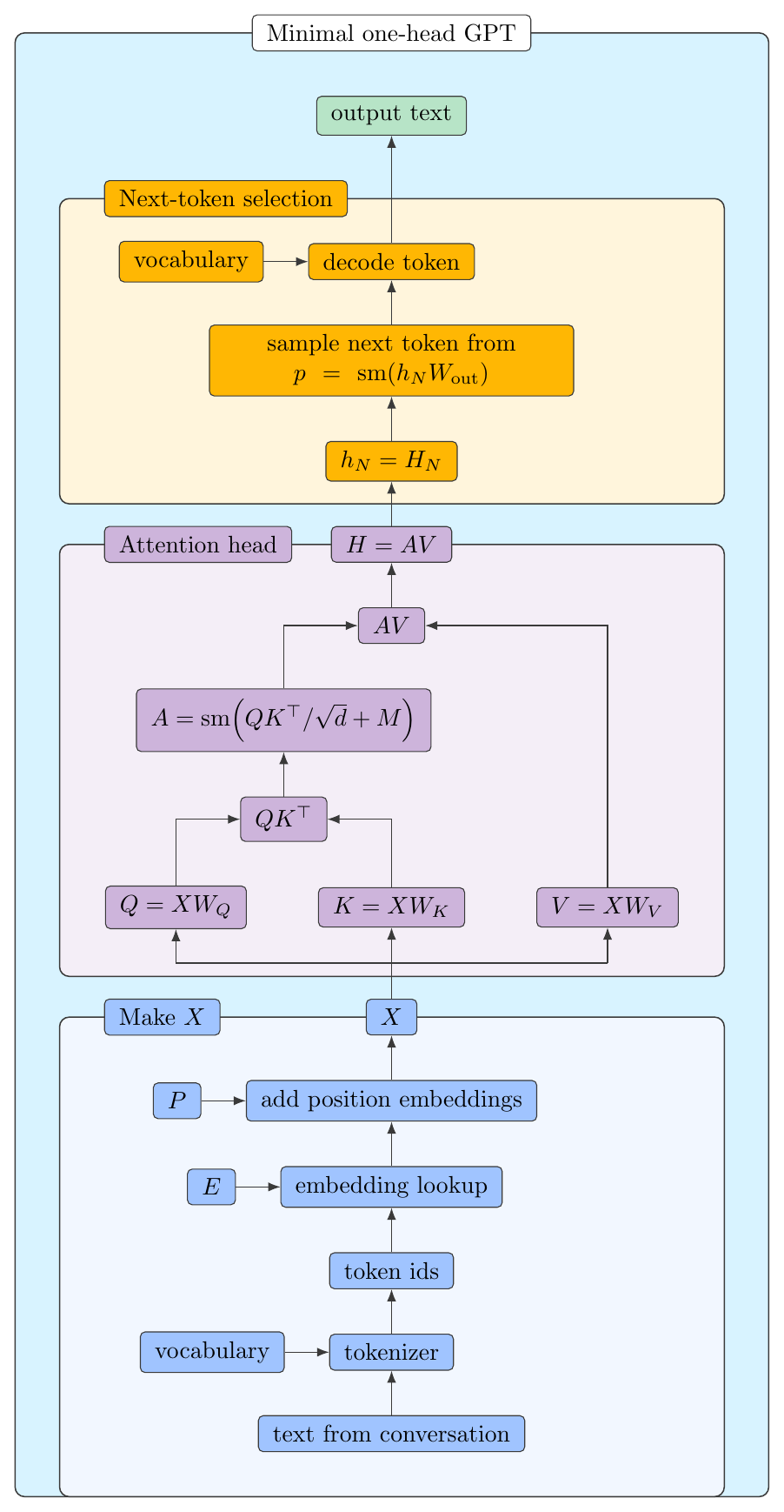
Read Fig. 8.1 from bottom to top. The lower box, Make \(X\), starts with the text from the conversation. It tokenizes this text with the vocabulary, looks up the corresponding rows of \(E\), adds the position embeddings from \(P\), and produces the context matrix \(X\). The attention-head box then takes \(X\) as input. It forms \(Q=XW_Q\), \(K=XW_K\), and \(V=XW_V\), builds the attention matrix \(A\), and produces the head output \(H=AV\). The next-token-selection box uses the last row \(H_N \in \R^{d}\) of \(H\), because this row corresponds to the end of the current context. With (8.3.2) we compute the score \(s\), using \(H_N\) as the summary vector \(h\). From there, the remaining steps are exactly those of the list in Section 8.1.

Fig. 8.2 shows how the one-head GPT is extended to a single transformer block with several heads. The input side is now collapsed to the single box \(X\), and the next-token-selection box is also collapsed: their internal details are exactly the ones from Fig. 8.1. The new part is the transformer in between.

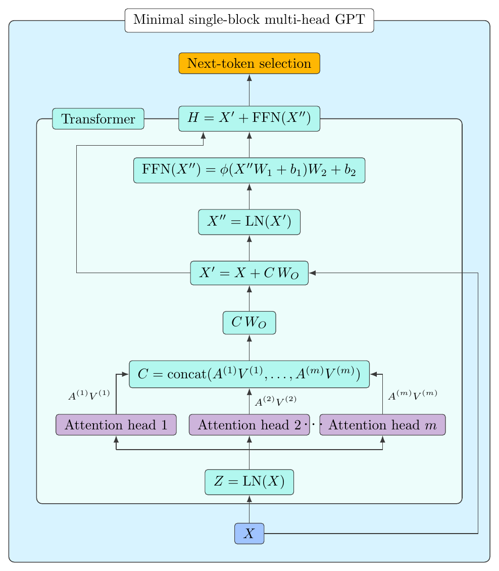
The input \(X\) is passed through layer normalization²⁷²⁷Wikipedia: Normalization (machine learning). before it enters the attention heads. Write

\begin{align*} Z=\LN{X}, \end{align*}

where

\begin{align*} z_{ik} &= \gamma_{k}\frac{x_{ik}-\bar x_i}{\sigma_i} +\beta_{k}, &\bar x_i &= \frac1d\sum_{k=1}^d x_{ik}, & \sigma_i^{2} &= \frac{1}{d}\sum_{k=1}^d (x_{ik}-\bar x_i)^2. \end{align*}

Thus, besides the standard normalization, transformers²⁸²⁸Layer normalization is less important in a single-layer toy GPT than in a real GPT. Real GPTs stack many transformer blocks, so repeated transformations can make scales drift; normalization keeps the row vectors on a comparable scale. usually include the learned parameters \(\gamma_k\) and \(\beta_k\) to make the normalization less rigid: if coordinate \(k\) should be larger, smaller, or shifted after standardization, training can pick this up.

Why do this before attention?²⁹²⁹Placing the normalization before each sublayer, as we do, is the pre-norm convention of GPT-2 and later models. The original Transformer instead normalized after the residual addition (post-norm). Both appear in the literature; pre-norm turns out to be easier to train for deep stacks. Attention scores are built from inner products. If the row scales drift after several transformations, then an inner product can become large because a row has a large norm, not because the tokens are especially relevant to each other. With this scaling, attention heads see vectors on a comparable scale.

After layer normalization, \(Z\) is sent to \(m\) attention heads in parallel.³⁰³⁰This is another reason not to assign much meaning to the term value matrix. If the value matrix were capable of selecting what is “of value” in a text, then a single attention head would suffice. Empirically, GPTs perform better when several such heads are used. Heuristically, since each head has its own matrices, each head is free to pick up different kinds of relation between tokens.³¹³¹One sometimes reads explanations in human terms, such as: one head attends to emotion, another to meaning. In my opinion, this is misleading. We do not know in such simple terms what individual heads learn. What we do know is that the trained GPT, as a whole, can produce text or computer code that is helpful to us. In head \(r\), the model forms its own queries, keys, and values,

\begin{align*} Q^{(r)} &= ZW_Q^{(r)}, & K^{(r)} &= ZW_K^{(r)},& V^{(r)} &= ZW_V^{(r)}. \end{align*}

It then computes its own causal attention matrix \(A^{(r)}\)³²³²With one change: the scaling inside the softmax is now \(\sqrt{d_h}\) instead of \(\sqrt d\), because the per-head queries and keys have \(d_h\) components. and produces \(A^{(r)}V^{(r)}\).

As the \(m\) heads have produced \(m\) separate answers for each token position, the head outputs are concatenated: \[ C=\operatorname{concat}(A^{(1)}V^{(1)},\ldots,A^{(m)}V^{(m)}). \] We want \(C\) to be an \(N\times d\) matrix, because those dimensions are expected by the rest of the model. Therefore the learned matrices of each head have dimensions \[ W_Q^{(r)},W_K^{(r)},W_V^{(r)}\in\R^{d\times d_h}, \] where \(d_h=d/m\).³³³³In standard implementations \(d\) is chosen as a multiple of \(m\), so that all heads can have the same integer width \(d_h=d/m\). After concatenation, the model mixes the outputs of the different heads by the learned linear map \(C W_O\).

As in neural networks, a skip connection adds the attention update to the current representation: \[ X'=X+C W_O. \] The attention block therefore learns a change to \(X\), not a complete replacement of \(X\).

We remark in passing that the sum \(X + CW_O\) is not normalized: under the pre-norm convention adopted above, normalization is applied to the input of each sublayer, never to the residual sum itself.

The matrix \(X'\) is normalized again and sent through a feed-forward network:³⁴³⁴This step was omitted in the one-head GPT because that example was meant to show the smallest attention-based prediction mechanism. That model still contains nonlinear operations, for instance the softmax in attention and the final softmax that turns token scores into a pmf, but it does not contain this extra learned row-wise neural-network layer. \[ X''=\LN{X'},\qquad \operatorname{FFN}(X'')=\phi(X''W_1+b_1)W_2+b_2. \] This is the ordinary neural-network part of the transformer block: first an affine transformation \(X''W_1+b_1\), then a componentwise nonlinearity \(\phi\),³⁵³⁵GPT uses the GELU. and then another affine transformation. The attention step and the feed-forward step therefore do different jobs. Attention mixes information between token positions: each row can use information from earlier rows. The feed-forward network works row by row, so each token position gets a nonlinear transformation of the information that attention has collected. It is common to expand each row temporarily to dimension \(4d\): then \(W_1\in\R^{d\times 4d}\) and \(W_2\in\R^{4d\times d}\). The first matrix gives the nonlinearity \(\phi\) more coordinates³⁶³⁶Empirically this larger intermediate dimension turns out to work well in transformer architectures. to act on; the second matrix maps back to dimension \(d\).

Finally, the feed-forward update is added back through a residual connection: \[ H=X' + \operatorname{FFN}(X''). \] The single output matrix \(H \in \R^{N\times d}\) is now ready for the same next-token-selection box used in the one-head GPT.

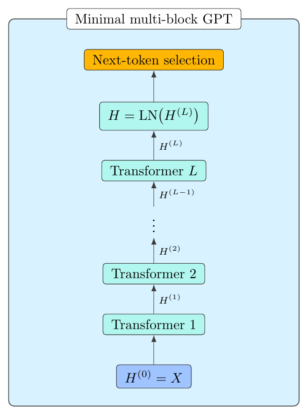
The full model applies \(L\) such transformer blocks³⁷³⁷These are the layers of neural networks. in turn, each with its own matrices, as shown in Fig. 8.3. We write \(H^{(0)}=X\). Transformer block \(l\) takes \(H^{(l-1)}\) as input and returns \(H^{(l)}\). After the last block, GPTs usually apply one more layer normalization, \[ H=\LN{H^{(L)}}. \] This final matrix \(H\) is sent to the same next-token-selection box used in the one-head GPT.

Now that the architecture is complete, one remark on the word transformer is in order. The original transformer of Vaswani et al.³⁸³⁸Wikipedia: Attention Is All You Need. was built for machine translation and consists of two coupled stacks of blocks, one for the source language, the other for the target language. A GPT has no separate source text to encode, so it needs no encoder. For this reason the GPT architecture is called decoder-only.