Regression problems aim to predict numerical values such as a price, a travel time, or a demand level.⁹⁹Wikipedia: Regression analysis. Therefore, in a regression problem, \(\Yset=\Aset=\R\), and the decision map \(d\) and label-lifting map \(r\) are identity maps.¹⁰¹⁰In classification problems, this is no longer the case.

We next consider two common regression losses: squared loss and absolute loss. For each loss, we first derive the Bayes predictor, then find the best predictors within the constant and affine model classes. Replacing population risk by training risk gives practical fitting procedures: squared loss leads to the sample mean and ordinary least squares, while absolute loss leads to sample medians and least absolute deviations regression.

The most common loss is squared loss, \[ \lscr(y, \hat y) = (y-\hat y)^2. \] The empirical average of squared loss over a list \(\Sset\) is called the mean squared error (MSE).¹¹¹¹Wikipedia: Mean squared error. In practice one often reports the root mean squared error (RMSE), the square root of the MSE, which has the same units as \(y\).

To find the optimal rule for this loss, suppose we know \(F_{X,Y}\) and may choose any prediction function. As a first step, we decompose the squared risk in a way that will be useful throughout this section. It separates the part of the error that can be reduced by choosing a better prediction rule from the variation in \(Y\) that remains once \(X\) is known.

Proof

Split the prediction error at \(m\):

\begin{align*} \E{(Y-f(X))^{2}} &= \E{\rb{\rb{Y-m(X)} + \rb{m(X)-f(X)}}^{2}} \\ &= \E{\rb{m(X)-f(X)}^{2}} + 2\E{\rb{m(X)-f(X)}\rb{Y-m(X)}}\\ &\quad + \E{\rb{Y-m(X)}^{2}}. \end{align*}

By conditioning on \(X\) in the middle term,

\begin{align*} \E{\rb{m(X)-f(X)}\rb{Y-m(X)} \given X} = \rb{m(X)-f(X)} \E{Y-m(X) \given X}= 0, \end{align*}

because \(m(X) = \E{Y \given X}\). With respect to the third term, conditioning on \(X\) yields

\begin{align*} \E{\rb{Y-m(X)}^{2}\given X} &= \E{Y^{2}\given X} - 2m(X)\E{Y\given X} + m(X)^{2}\\ &= \E{Y^{2}\given X} - m(X)^{2}. \end{align*}

From the definition of conditional variance

\begin{align*} \V{Y\mid X} &= \E{ (Y-\E{Y\mid X}\mid X} = \E{Y^{2}\mid X} - m(X)^{2}. \end{align*}

Taking expectations completes the proof.

The Bayes regressor under squared loss now follows easily.

Fitting the best constant function requires minimizing \(\E{(m(X) -c)^2}\) in (3.2.1). Expanding the square and using that \(\E{m(X)} = \E Y\), gives

\begin{align*} \E{m(X)^{2}} +c (c-2 \E Y). \end{align*}

This is minimal at \(c^* = \E Y\), and then the risk \(R(c^*)\) becomes

\begin{align*} c^{*} &= \E Y, & R(c^*) &= \E{\V{Y\mid X}} + \E{m(X)^{2}} - (\E Y)^{2} = \V Y, \tag{3.2.2} \end{align*}

where the last step follows from Eve’s law.

To obtain the empirical risk minimizer and minimal empirical risk, we replace \(F_{X,Y}\) by the measure induced by \(\Tset\) to get

\begin{align*} \hat c &= \hat y = \frac{1}{|\Tset|}\sum_{(x,y)\in\Tset}y, & \hat R_{\Tset}(\hat c) &= \frac{1}{|\Tset|}\sum_{(x,y)\in\Tset}(y-\hat c)^2. \tag{3.2.3} \end{align*}

For an affine prediction rule the population problem is to minimize the approximation term in (3.2.1), since the irreducible-noise term does not depend on the affine parameters:

\begin{align*} \E{\rb{m(X)-f_{\beta_0,\beta}(X)}^2} &= \E{\rb{m(X)-\beta_0-\ip{\beta,X}}^2}. \end{align*}

Setting the partial derivatives wrt \(\beta\) and \(\beta_0\) to zero gives the population normal equations:

\begin{align*} \beta_0 + \ip{\beta, \E{X}} &= \E Y,\\ \E{\rb{m(X)-\beta_0-\ip{\beta,X}}X(j)} &= 0, \qquad j=1,\ldots,p. \end{align*}

Replacing \(F_{X,Y}\) by the measure induced by \(\Tset\) gives

\begin{align*} \hat\beta_0 + \ip{\hat\beta,\hat x} &= \hat y,\\ \sum_{(x,y)\in\Tset}\rb{y-\hat\beta_0-\ip{\hat\beta,x}}x(j) &= 0, \qquad j=1,\ldots,p. \end{align*}

These solve the ordinary least squares (OLS) problem:

\begin{align*} (\hat\beta_0,\hat\beta) &\in\argmin_{\beta_0,\beta}\hat R_{\Tset}(f_{\beta_0,\beta}), \tag{3.2.4} \\ \hat R_{\Tset}(f_{\beta_0,\beta}) &=\frac{1}{|\Tset|}\sum_{(x,y)\in\Tset} \rb{y-\beta_0-\ip{\beta,x}}^2. \tag{3.2.5} \end{align*}

Restricting the affine class to \(\beta=0\) recovers the constant class: the population equation gives \(\beta_0^*=\E{Y}\), and the sample equation gives \(\hat\beta_0=\hat c\) of (3.2.3).

Bias and variance are two forms of error that appear through the approximation of \(m(x)\) by the empirical risk minimizer \(\hat f_\Tset\), (3.1.5). Write \[ \bar f(x)=\EE{\Tset}{\hat f_{\Tset}(x)} \] for the average prediction at \(x\) over the iid training samples that can obtained from \(F_{XY}\). The bias is \(\bar f(x)-m(x)\): the systematic discrepancy between the average fitted prediction and the conditional mean. The variance measures how much the fitted prediction changes when we draw a new training sample.

There are two sources of randomness to distinguish. The training sample determines the fitted rule; a new observation \((X^0,Y^0)\), independent of \(\Tset\) and with distribution \(F_{X,Y}\), determines where and against which outcome we evaluate that rule.

Proof

Fix \(x\). In the first term in (3.2.1) add and subtract the average fitted prediction to get \[ m(x)-\hat f_{\Tset}(x) =\bigl(m(x)-\bar f(x)\bigr) +\bigl(\bar f(x)-\hat f_{\Tset}(x)\bigr). \] Squaring, expanding and taking the expectation over \(\Tset\) gives

\begin{align*} (m(x)-\bar f(x))^2 +2(m(x)-\bar f(x)) \EE{\Tset}{\bar f(x)-\hat f_{\Tset}(x)} +\EE{\Tset}{(\bar f(x)-\hat f_{\Tset}(x))^2}. \end{align*}

The cross term vanishes: by the definition of \(\bar f\), \[ \EE{\Tset}{\bar f(x)-\hat f_{\Tset}(x)} =\bar f(x)-\EE{\Tset}{\hat f_{\Tset}(x)}=0. \] The third term is the variance of the fitted prediction across training samples.

Taking the expectation over a new observation \(X\), combining this with (3.2.1), and using the independence of \(X\) and \(\Tset\) proves the result.

Feature selection affects both bias and variance. Suppose for this paragraph that the feature coordinates are uncorrelated, so that leaving one out does not disturb the estimates of the others. A feature with \(\beta_{j}=0\) has no contribution to the conditional mean, so estimating its coefficient adds variance without reducing bias. Omitting it therefore lowers the variance of the fitted rule without increasing bias. Omitting a feature with \(\beta_{j}\neq0\) leaves its contribution \(\beta_{j}x(j)\) inside the residual, which raises the residual variance, and every remaining coefficient is estimated against that larger noise; omitting it therefore raises the variance of the remaining estimates and introduces bias. Feature selection aims to retain useful features and omit those that add only estimation noise. The lasso in Section 3.5 is one method for selecting features.

Nominal classification problems have categorical labels without a natural order. This means that for \(K\)-class nominal classification, the label lies in the set¹⁴¹⁴It is common to assume that labels like ’red’ and ’green’ are already converted to numbers. \[ \Yset = \Kset=\set{1,\ldots,K}. \] Besides the prediction \(\hat y\) for the label \(y\), we will be concerned with probability prediction \[ \hat p = (\hat p_1,\ldots,\hat p_K) \in \Delta_K, \] where \(\Delta_{K}\) is the /probability simplex \[ \Delta_K = \set{p\in\R^K : p_k\geq 0,\ \sum_{k=1}^{K} p_k = 1}. \] Here \(\hat p_k\) is interpreted as the predicted probability of class \(k\).

Throughout this section the prediction set \(\Aset=\Delta_K\), and the fitted rule returns \(\hat a = \hat p\). When a single class has to be returned based on \(\hat p\), the decision map is the argmax rule¹⁵¹⁵This rule is the same as majority vote when \(\hat p\) is the vector of class frequencies of a sample list \(\Sset\): the label with the highest probability is then the most frequent one.

\begin{align*} \hat y = d(\hat p) \in \argmax_{k} \hat p_k. \tag{3.3.1} \end{align*}

In the other direction, the observed class \(y\) is lifted into the simplex by the one-hot encoding of \(y\), \[ a = q = r(y), \qquad q_k=\1{y=k}, \] which puts probability one on the observed class and zero on all others.¹⁶¹⁶Observe that, as required, \(d(r(y))=y\).

For any list \(\Sset\) whose labels lie in \(\Kset\), \(\Sset_{k} = \qb{(x,y)\in\Sset : y=k}\) is the sublist of samples of class \(k\). Write \(p\) for the vector with components¹⁷¹⁷That is, the marginal probabilities. \(p_{k} = \P{Y=k}\), and \(p(x)\) be the vector of conditional class probabilities with components \(p_{k}(x) = \P{Y=k \mid X=x}\). For the non-empty training list \(\Tset\), write \(\Tset_k=\qb{(x,y)\in\Tset:y=k}\) and \(\hat p_k=|\Tset_k|/|\Tset|\).

Zero-one loss compares samples based on class:

\begin{align*} \lscr(a, \hat a) = \lscr(q, \hat p) = \1{d(q) \neq d(\hat p)} = \1{y \neq d(\hat p)}. \tag{3.3.2} \end{align*}

The next numerical example shows an important problem with zero-one loss. Take two classes, \(K=2\), and suppose the observed class is \(y=1\), which converts into the one-hot vector \(q=(1,0)\). Compare the two probability predictions

\begin{align*} \hat p^{A} &= (0.51,0.49), & \hat p^{B} &= (0.99,0.01). \end{align*}

The two predictions receive the same zero-one loss, but this loss does not show confident the probability vector is. As a consequence, optimizing under zero-one loss is difficult because small changes in the probabilities often leave the predicted label unchanged.

For any rule \(f:\Xset\to\Delta_K\) write \(g=d\circ f : \Xset \to \Kset\). Then for the conditional risk

\begin{align*} \E{\lscr(r(Y),f(X))\mid X=x} &= \E{Y \neq g(X) \mid X=x} \\ &= \P{Y \neq g(X) \mid X=x} \\ &= 1 - \P{Y = g(X) \mid X=x}. \end{align*}

Therefore, \[ \argmin_{g} \E{\1{ Y \neq g(X)|X=x}} = \argmax_{k\in K} \P{Y=k |X=x}. \] Using (3.3.1), we see that the Bayes classifier \(f^*\) has components

\begin{align*} f^{*}_{k}(x) = \P{Y=k \mid X=x} = p_{k}(x). \tag{3.3.3} \end{align*}

For a constant predictor \(d(f(x)) =k\), the loss becomes

\begin{align*} R(f) = \E{Y\neq k} = 1-\P{Y=k}. \end{align*}

Thus the best constant predictor is the majority class and the risk is the misclassification rate,

\begin{align*} \hat y &\in \argmax_{k} |\Tset_{k}|, & \hat R_{\Tset}(r(\hat y)) &= 1 - \max_{k} \hat p_{k}. \tag{3.3.4} \end{align*}

The Brier loss¹⁸¹⁸Wikipedia: Brier score.

\begin{align*} \lscr(q,\hat p) = \sum_{k=1}^{K}(q_k-\hat p_k)^2 \tag{3.3.5} \end{align*}

compares the one-hot representation \(q=r(y)\) to the prediction \(\hat p\).

A numerical example shows the advantage of Brier loss over zero-one loss. Take two classes, \(K=2\), and suppose the observed class is \(y=1\), which converts into the one-hot vector \(q=(1,0)\). Compare the two probability predictions

\begin{align*} \hat p^{A} &= (0.51,0.49), & \hat p^{B} &= (0.99,0.01). \end{align*}

For the Brier loss, both probability components enter the loss. For \(\hat p^{A}\),

\begin{align*} \lscr(q,\hat p^{A}) &= (q_1-\hat p^{A}_{1})^{2} + (q_2-\hat p^{A}_{2})^{2} \\ &= (1-\hat p^{A}_{1})^{2} + (0-\hat p^{A}_{2})^{2} \\ &= (1-0.51)^2 + (0-0.49)^2 \\ &= 0.49^2 + 0.49^2 \\ &\approx 0.48. \end{align*}

For \(\hat p^{B}\),

\begin{align*} \lscr(q,\hat p^{B}) &= (q_1-\hat p^{B}_{1})^{2} + (q_2-\hat p^{B}_{2})^{2} \\ &= (1-\hat p^{B}_{1})^{2} + (0-\hat p^{B}_{2})^{2} \\ &= (1-0.99)^2 + (0-0.01)^2 \\ &= 0.01^2 + 0.01^2 \\ &= 0.0002. \end{align*}

Thus the second prediction receives a much smaller Brier loss, because its probability vector is closer to the one-hot vector for the observed class.

The maximum value \(2\) is attained when the prediction puts all probability on the wrong class.

For the Bayes predictor we split the risk in a similar way as Th. 3.2.1. As the \(k\)th component of \(r(Y)\) is \(\1{Y=k}\), the Brier loss becomes

\begin{align*} \E{\lscr(r(Y), f(X))} = \E{\sum_{k=1}^{K}\rb{\1{Y=k} - f_{k}(X)}^{2}} = \sum_{k=1}^{K} \E{\rb{\1{Y=k} - f_{k}(X)}^{2}}. \end{align*}

To minimize this, we can minimize each of the terms in the summation, which allows us to apply Th. 3.2.1 to each term separately with \(\1{Y=k}\) in the role of \(Y\) for the \(k\)th term. By straight comparision, its conditional expectation is \(\E{\1{Y=k}\given X} = p_{k}(X)\). The conditional variance¹⁹¹⁹An indicator with success probability \(p\) has variance \(p(1-p)\). is \(\V{\1{Y=k}\given X} = p_{k}(X)\rb{1-p_{k}(X)}\). Summing the variances over \(k\) and using that the \(p_{k}(x)\) add up to one,

\begin{align*} \sum_{k=1}^{K} p_{k}(x)\rb{1-p_{k}(x)} = 1 - \sum_{k=1}^{K} p_{k}(x)^{2}. \end{align*}

Summarizing:

From the above and Cor. 3.2.2 we obtain the following corollary.

A constant vector as a predictor has the form \(f_c(x)=c \in \Delta_{\Kset}\). As each term \(f_k\) is constant, we can use (3.2.2) term by term. Again, with \(\1{Y=k}\) in the role of \(Y\) for the \(k\)th term, the optimal constant is \(\E{\1{Y=k}} = p_k\) and the variance is \(\V{\1{Y=k}} = p_k(1-p_k)\). Thus the best-in-class predictor and its risk are

\begin{align*} c^{*} &=p, & R(c^{*})&=1-\sum_{k=1}^{K}p_k^2. \end{align*}

Replacing the marginal probabilities by sample frequencies gives

\begin{align*} \hat c^{*}&=\hat p, & \hat R_{\Tset}(c^{*}) &= 1 - \sum_{k=1}^{K} \hat p_{k}^{2}. \tag{3.3.6} \end{align*}

If several training samples have exactly the feature vector \(x\), we can estimate \(m(x)\) by averaging their outcomes. For continuously distributed features, exact matches to a specified \(x\) generally do not occur. Instead, we can average outcomes at feature vectors near \(x\), using the idea that their conditional means should also be close.

Choose a number of neighbors \(k\), with \(1\leq k\leq n\), and measure closeness by Euclidean distance: \[ \norm{x_i-x}_2 =\left(\sum_{j=1}^p (x_i(j)-x(j))^2\right)^{1/2}. \] Let \(i_1(x),\ldots,i_n(x)\) be the training indices ordered by increasing distance to \(x\). Break equal-distance ties by the original sample index, so that the first \(k\) indices always identify exactly \(k\) samples, including repeated samples when present. The \(k\)-nearest-neighbor (KNN)²⁰²⁰We use lowercase \(k\) for the number of neighbors; uppercase \(K\) continues to denote the number of classes. prediction is

\begin{align*} \hat f_{k,\Tset}(x)=\frac{1}{k}\sum_{a=1}^k y_{i_a(x)}. \tag{3.4.1} \end{align*}

This is precisely the fitted constant of (3.2.3), but fitted to the local list \(\Tset_k(x)=[(x_{i_1(x)},y_{i_1(x)}),\ldots,(x_{i_k(x)},y_{i_k(x)})]\). The list changes with the prediction point. The resulting rule can therefore follow a nonlinear conditional mean even though each individual prediction is obtained by fitting a constant.

\begin{algorithm}
\caption{Predict by averaging the outcomes of exactly \(k\) nearest training samples.}
\begin{algorithmic}
\State \textbf{Input:} a non-empty training list $\Tset$, a feature vector $x$, and an integer $1\leq k\leq|\Tset|$.
\State \textbf{Output:} a numerical prediction at $x$.
\Procedure{KnnPredict}{$\Tset,x,k$}
    \State Order the indices $i_1,\ldots,i_n$ by increasing $\norm{x_i-x}_2$, breaking ties by index.
    \Return $\pr{Average}([y_{i_1},\ldots,y_{i_k}])$
\EndProcedure
\end{algorithmic}
\end{algorithm}

Distances depend on the units of the features. A coordinate measured in euros can dominate one measured in kilometers even if both are useful. One common choice is to center each feature and divide it by its training standard deviation before calculating distances. The same transformation, with the same fitted means and standard deviations, is then applied to new inputs. For \(1\leq j\leq p\), let²¹²¹We apply the last transformation only when \(\sigma(j)>0\); constant features can be omitted.

\begin{align*} \mu(j)&=\frac{1}{n}\sum_{i=1}^{n}x_i(j),& \sigma(j)&=\sqrt{\frac{1}{n}\sum_{i=1}^{n}(x_i(j)-\mu(j))^2},& \tilde x_i(j)&=\frac{x_i(j)-\mu(j)}{\sigma(j)}. \tag{3.4.2} \end{align*}

A numerical example demonstrates clearly the effect of \(k\). Consider the conditional mean

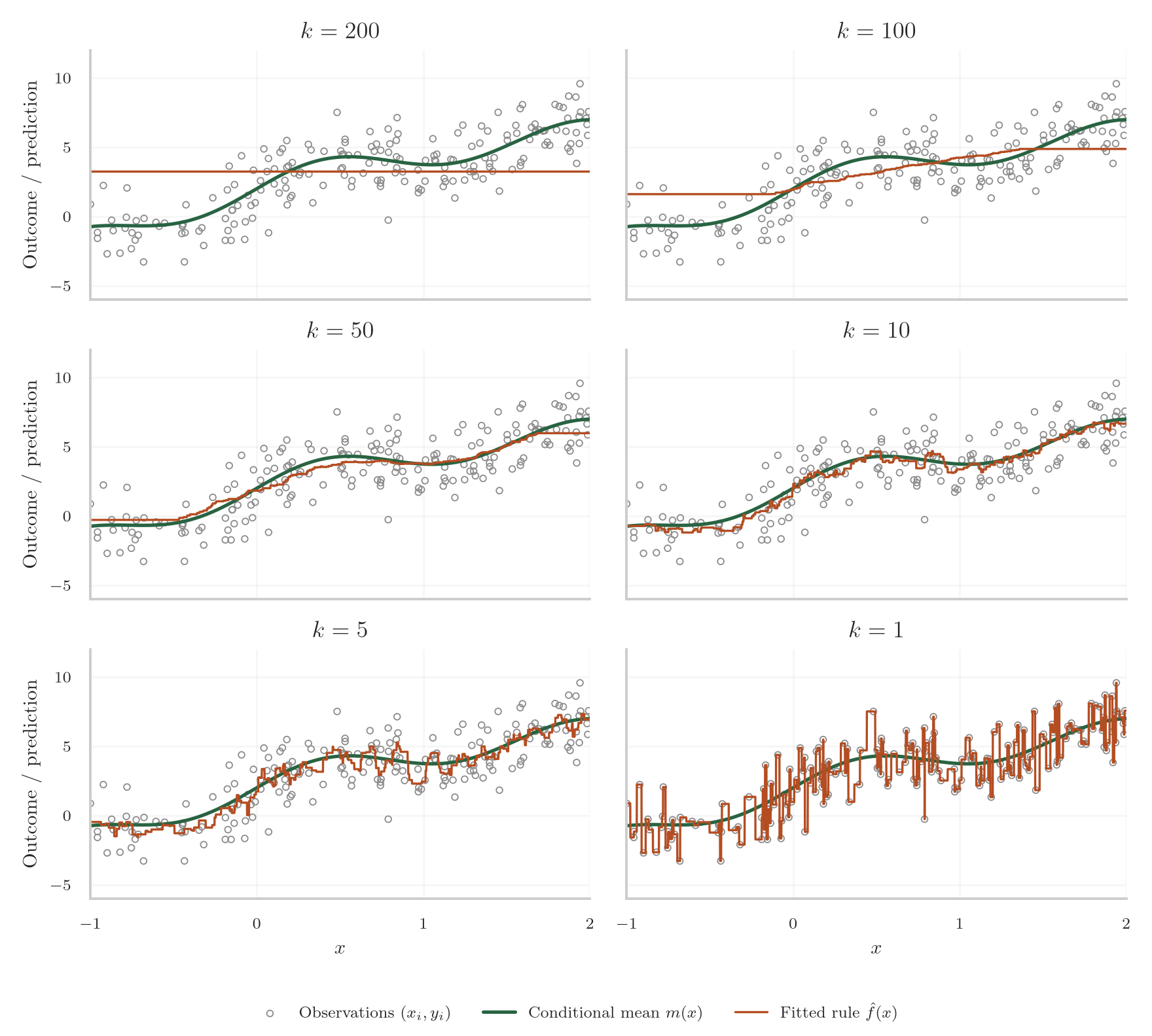
\begin{align*} m(x)=2-\frac{1}{2}x^2+3x+\sin(4x),\qquad -1\leq x\leq2. \tag{3.4.3} \end{align*}

Generate \(n=200\) independent samples according to \[ X_i\sim\operatorname{Unif}(-1,2),\qquad Y_i=m(X_i)+\varepsilon_i,\qquad \varepsilon_i\sim\mathcal N(0,1.5^2), \] with the noises independent of the inputs and of one another. Then \(\E{Y_i\given X_i=x}=m(x)\).²²²²Because this is a constructed example, we know \(m\); in an application we only observe the pairs \((x_i,y_i)\).

Fig. 3.1 compares \(k=200,100,50,10,5,1\) on the same sample. At \(k=200\) the rule is constant and cannot follow the trend or the oscillations. At \(k=1\), the fitted rule reproduces each training outcome, including its noise, which is clearly overfitting.

When the number of features \(p\) is large, e.g. \(p\geq 10\), the nearest neighbors of \(x\) are no longer close to \(x\). Two computations show this for samples that are uniformly distributed on \([0,1]^p\).

First, consider a sub-cube with sidelength²³²³Hence with volume \(a^p\). \(a\) contains a fraction \(s\) of the samples. Then, \(a = s^{1/p}\). For \(s=0.01\) and \(p=10\) this side length is \(0.01^{1/10}\approx 0.63\): a neighborhood that holds 1% of the samples spans 63% of the range of each feature.

Second, let \(X\) and \(X'\) be independent uniform points in \([0,1]^p\). Then

\begin{align*} \E{\norm{X-X'}_2^2} &= \sum_{j=1}^{p}\E{(X(j)-X'(j))^2} = \frac{p}{6}, \tag{3.4.4} \\ \V{\norm{X-X'}_2^2} &= \sum_{j=1}^{p}\V{(X(j)-X'(j))^2} = \frac{7p}{180}, \tag{3.4.5} \end{align*}

where the second line uses that the coordinate differences are independent. The squared coefficient of variation²⁴²⁴The variance divided by the squared mean. is

\begin{align*} \frac{\V{\norm{X-X'}_2^2}}{\E{\norm{X-X'}_2^2}^{\,2}} = \frac{7}{5p}. \tag{3.4.6} \end{align*}

Thus, as \(p\) grows, the variation of squared distances relative to their mean becomes small: all points lie roughly equally far away. The \(k\) nearest samples are then barely closer to \(x\) than the other samples, so their average says little more about \(m(x)\) than an average over arbitrary samples. Yet using all \(n\) observations is also undesirable, since it gives the global constant predictor.

This is the curse of dimensionality: local averaging becomes difficult in high dimension. An alternative restricts the rule to a class \(\Fset\) with a fixed number of parameters. All \(n\) samples then contribute to fitting each parameter, not only the \(k\) samples nearest to \(x\).

Polynomial regression is one such class. For a nonnegative integer degree \(q\), define

\begin{align*} \Fset_q =\left\{f_\beta:f_\beta(x)=\beta_0+\sum_{j=1}^q\beta_jx^j,\ \beta\in\R^{q+1}\right\}. \tag{3.4.7} \end{align*}

The cases \(q=0\) and \(q=1\) recover the constant and affine classes for one numerical input. For \(q>1\), the rule is generally nonlinear in \(x\), but remains affine in the transformed features \((x,x^2,\ldots,x^q)\) and linear in the coefficients. Fitting therefore uses the same least-squares method as before: \[ \hat\beta\in\argmin_{\beta\in\R^{q+1}} \frac{1}{n}\sum_{i=1}^n \left(y_i-\beta_0-\sum_{j=1}^q\beta_jx_i^j\right)^2. \] The coefficients \(\beta\) are parameters: least squares fits them for a given degree. The degree \(q\) is a hyperparameter: it fixes the class \(\Fset_q\) in which we fit.

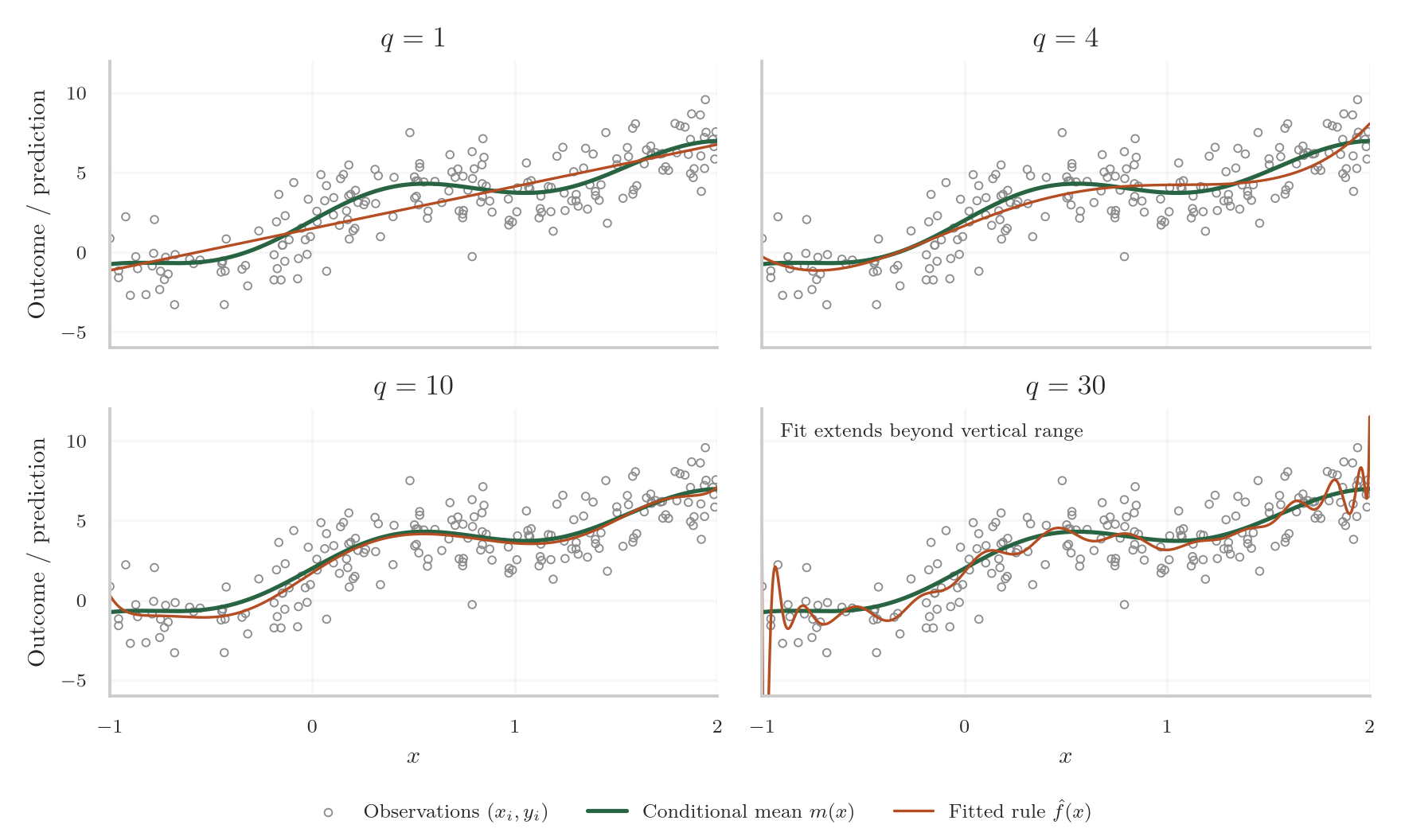
Fig. 3.2 compares degrees \(q=1,4,10,30\) on the same observations used for KNN. An affine rule, \(q=1\), cannot follow the oscillations in \(m\). A polynomial of degree \(q\) has at most \(q-1\) turning points, so a higher degree can improve the approximation of \(m\), but it also lets the fit respond more strongly to the noise in the sample. The \(q=10\) fit follows \(m\) closely; the \(q=30\) fit adds oscillations, especially near the endpoints.

Choosing and assessing a prediction rule takes three steps. First, we select a function class \(\Fset\) over which we fit. A function in \(\Fset\) is specified by hyperparameters and parameters. For instance, for the union of the polynomial classes (3.4.7), the degree \(q\) is a hyperparameter and the coefficients \(\beta_0,\ldots,\beta_q\) are the parameters. Here we discuss how to tune the hyperparameters and the coeficients and assess how well the final result would do on a new observation \(X\). To tune a hyperparameter, we fix in advance a finite set of values to compare, for instance the degrees \(\Gamma = \set{0,1,\ldots,30}\). Each value in this set is a candidate, and the rule fitted at a candidate is a candidate rule.

For independent observations from a common population, we can randomly divide the available sample into three disjoint lists:

• The training list \(\Tset\): used to fit candidate rules.
• The validation list \(\Vset\): used to select a candidate.
• The test list \(\Sset_{\mathrm{test}}\): kept aside to assess the final rule after selection and fitting are complete.

Splitting the samples into these subsets affects both fitting accuracy and evaluation precision: more training data can improve a fitted rule, while more evaluation data make its measured risk more precise. There is no single split proportion that is appropriate for every sample size and prediction problem.

Let \(\Gamma\) be a finite collection of candidate settings and let \(\hat f_{\gamma,\Tset}\) be the rule fitted with setting \(\gamma\). Now we use the validation set \(\Vset\) to find the best \(\gamma\). Writing the risk on the validation set as \(\hat R_\Vset(\hat f_{\gamma, \Tset})\),²⁸²⁸Note: each candidate is fitted without using the validation observations. the best candidate is

\begin{align*} \hat\gamma\in\argmin_{\gamma\in\Gamma} \hat R_{\Vset}(\hat f_{\gamma,\Tset}). \tag{3.6.1} \end{align*}

After choosing \(\hat\gamma\), we can refit on the concatenated list \( \Dset=\Tset+\Vset. \) The final rule is then \(\hat f_{\hat\gamma,\Dset}\).

Finally, we use the test list to assess the final rule. Its test risk \[ \hat R_{\Sset_{\mathrm{test}}}(\hat f_{\hat\gamma,\Dset}) \] is the average loss of \(\hat f_{\hat\gamma,\Dset}\) over the test samples. The test samples are used neither to fit the parameters nor to select \(\hat\gamma\). For the final rule they are therefore new observations, and the test risk estimates its risk \(R(\hat f_{\hat\gamma,\Dset})\) on a new observation \((X,Y)\). Since the test risk is an average of losses on independent samples, a larger test list gives a more precise estimate.

Preprocessing is part of fitting. Means and standard deviations used to scale inputs must be estimated on the training part, then applied unchanged to the validation part. Feature selection, missing-value imputation, and other transformations estimated from data must follow the same procedure. Allowing the validation or test data to influence fitting is called data leakage.

In the procedure above the candidate rules are fitted on \(\Tset\) only, and \(\Vset\) is never used for this purpose. Cross-validation divides \(\Dset=\Tset+\Vset\) instead into several parts. Each part serves once as validation list, while the rules are fitted on the other parts. Every sample in \(\Dset\) is then used for fitting and for validation, but never both in the same fit.

Let \(N=|\Dset|\), and divide its sample indices into \(F\) disjoint non-empty folds \(\Iset_1,\ldots,\Iset_F\), usually of nearly equal size. For fold \(b\), write

\begin{align*} \Dset_b &=[(x_i,y_i):i\in\Iset_b],& \Dset_{-b} &= \Dset\setminus \Dset_{b} = [(x_i,y_i):i\notin\Iset_b]. \end{align*}

In \(F\)-fold cross-validation, we fit a candiate \(\gamma\) on \(\Dset_{-b}\) and we evaluate its risk on \(\Dset_b\).²⁹²⁹Use the same folds for every candidate, so their errors are compared on the same validation observations. Writing \(\hat f_{\gamma,\Dset_{-b}}\) for such a fit, the cross-validation criterion for candidate \(\gamma\) is

\begin{align*} \mathrm{CV}(\gamma) &=\frac{1}{N}\sum_{b=1}^F\sum_{i\in\Iset_b} \lscr(r(y_i),\hat f_{\gamma,\Dset_{-b}}(x_i)) \\ &=\sum_{b=1}^F\frac{|\Dset_b|}{N} \hat R_{\Dset_b}(\hat f_{\gamma,\Dset_{-b}}). \tag{3.6.2} \end{align*}

Every sample contributes one loss, from a rule fitted without that sample’s fold. The weights account for unequal fold sizes. Now select \[ \hat\gamma\in\argmin_{\gamma\in\Gamma}\mathrm{CV}(\gamma). \] Again, once \(\hat \gamma\) is computed, fit the model on \(\Dset\) for this candidate.

A special case is when \(F=N\); this is called leave-one-out cross-validation: each fit omits just one sample.

\begin{algorithm}
\caption{Select a setting by cross-validation and refit on all development data.}
\begin{algorithmic}
\State \textbf{Input:} a development list $\Dset$, candidate settings $\Gamma$, and $2\leq F\leq|\Dset|$.
\State \textbf{Output:} a selected setting and the final fitted rule.
\Procedure{CrossValidate}{$\Dset,\Gamma,F$}
    \State Divide the indices of $\Dset$ into folds $\Iset_1,\ldots,\Iset_F$.
    \For{$\gamma\in\Gamma$}
        \State $\mathrm{CV}(\gamma)\gets0$
        \For{$b=1,\ldots,F$}
            \State Fit all preprocessing and the rule at $\gamma$ on $\Dset_{-b}$.
            \State $\mathrm{CV}(\gamma)\gets\mathrm{CV}(\gamma)+
            \dfrac{|\Dset_b|}{|\Dset|}\hat R_{\Dset_b}(\hat f_{\gamma,\Dset_{-b}})$
        \EndFor
    \EndFor
    \State $\hat\gamma\gets$ a minimizer of $\mathrm{CV}(\gamma)$ over $\Gamma$
    \State Refit preprocessing and the rule at $\hat\gamma$ on all of $\Dset$.
    \Return $(\hat\gamma,\hat f_{\hat\gamma,\Dset})$
\EndProcedure
\end{algorithmic}
\end{algorithm}

The number of folds \(F\) affects cross-validation in three ways.

First, with equal folds, each fold rule is fitted on \(N(1-1/F)\) samples, while the final rule \(\hat f_{\hat\gamma,\Dset}\) is fitted on all \(N\). A rule fitted on fewer samples has a larger estimation error, so with cross validation we obtain usually less good predictors. Hence \(\mathrm{CV}(\gamma)\) tends to be somewhat larger than the risk of the rule fitted at \(\gamma\) on all of \(\Dset\).

Second, cross-validation fits every candidate \(F\) times, so \(F|\Gamma|\) fits in total, plus the final refit. Hence, CV increases the compuational load.

Third, the random variation of \(\mathrm{CV}(\gamma)\). Whatever \(F\), each sample of \(\Dset\) is validated exactly once, so \(\mathrm{CV}(\gamma)\) is always an average of \(N\) losses. What changes with \(F\) is how much the fold rules have in common. For large \(F\), any two fitting lists \(\Dset_{-b}\) share all but \(2N/F\) samples, so the fold rules are nearly the same rule. If that rule happens to be poor, all its losses are large together, and averaging them removes less of this chance variation than averaging over rules fitted on different samples. Taking \(F=5\) or \(F=10\) keeps the fold training size at 80 or 90 percent of \(N\), with 5 or 10 fits per candidate.